Sharding pgvector
If you find yourself working with embeddings, you’ve shopped around for a vector database. pgvector is a great option if you’re using Postgres already. Once you reach a certain scale (about a million arrays), building indices starts taking a long time. Some workarounds, like parallel workers, help, but you still need to fit the whole graph in memory.
The solution to lots of data is more compute, so we sharded pgvector. In this context, we’re specifically talking about sharding a vector index. Splitting tables between machines is easier. Our goal is to have fast and good recall: we want to quickly find matches when we search for them.
A bit of background
pgvector has two types of indexes: HNSW and IVFFlat. They are different ways to organize vectors in multi-dimensional space. HNSW builds a multi-layer graph that can be searched quickly, in O(log(n)) time. The trade-off is it takes a long time to build.
IVFFlat splits the vector space into parts, grouped around centroids, i.e., points in space that seem to be in the center of something. Finding that something is done using K-means, a machine learning (mathematical, really) algorithm for grouping arbitrary things. IVFFlat index is quick to build, but slower to search. Once the graph is split into parts, searching becomes roughly O(sqrt(n))). Lastly, to find centroids, you need to have a representative sample of your vectors beforehand. Centroids are specific to your data and are not generalizable.
Both of these algorithms work well when parts of the graph are hot and others cold. The hot area grows as your company does, since more users search for more stuff. Once the hot area exceeds your memory, things slow down. If your algorithm has a linear-time component, even searching in memory isn’t always as quick as you’d like.
Sharding the index
Using first principles, sharding a vector index means splitting it into parts. Stating the obvious is sometimes a good idea. When you say that out loud, IVFFLat becomes the obvious choice. It does that already. It splits embeddings into groups using K-means. That means, we can do the same thing for sharding. Except, instead of placing the parts on the same machine, let’s place them on multiple. When we search for a match, we can pick a host (or multiple), based on a query parameter.
To test this idea, we took a publicly available dataset from HuggingFace. It’s called Cohere/wikipedia and it’s an encoding of the entire English Wikipedia using an AI embedding model. It produces embeddings with 768 points, so our vector in Postgres is pretty large:
CREATE TABLE embeddings (
  title text,
  body text,
  embedding vector(768),
);
Wikipedia articles have a title and a body. The model generates a mathematical summary of what the article is about so we can easily find articles based on some context, provided by the user. This is called semantic search and it’s used everywhere, including Google.
With the table schema ready, the next step is to figure out the centroids. For this, we used scikit-learn. It’s super simple to use and has all the algorithms we need. After downloading a sample from HuggingFace (the dataset is split for us already), calculating K-means was pretty simple. I’ll save you the trouble of looking at code now. All of it is available in our GitHub repository.
Have you ever wondered what the summary of all human knowledge looks like on a graph? Here it is, reduced to 2 dimensions using PCA:
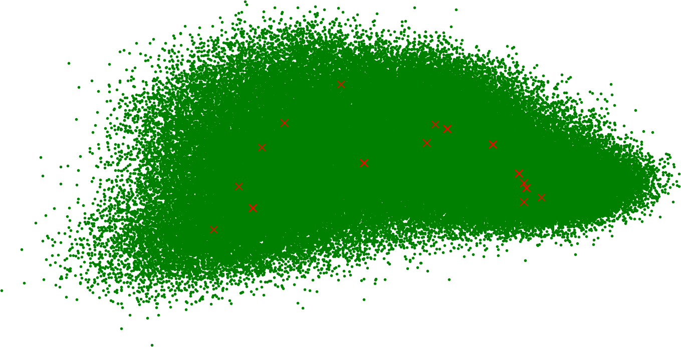
The little red x’s are centroids. We calculated 16 because it seems like a good number to start with. For our purposes, we need as many centroids as we have shards. If you know a data scientist, they will tell you how many is a good idea for your dataset.
Placement of data is important and we’ll cover it in a minute. For now, our sharding function is:
shards = pick(min(l2_distance(vector, centroids)) mod shards, probes)
Using Euclidean distance, we’re looking for the shards that have the centroids closest to the vector in the query. If you’re using pgvector already, you know it as the <-> operator or the vector_l2_ops index type.
Since we’re using IVFFlat, we know that 1 probe isn’t enough, so we pick multiple. You can configure how many you’d like in pgdog.toml. By default, we are setting it to sqrt(centroids), in our case, that’s 4. This is analogous to the ivfflat.probes setting in pgvector and improves recall, at the cost of compute utilization. The performance does not suffer that much, since the lookups are done in parallel over warm connections.
Adding support for vectors in PgDog was straightforward. We are using pg_query, a Rust crate that directly bundles the PostgreSQL query parser. PgDog can read all valid Postgres queries. When searching for a match, typically, you’re trying to rank vectors by distance. The closer they are to each other, the better the semantic match between data they represent.
To make this work, we parse the ORDER BY clause that contains the <-> operator and route it to the nearest shards to the parameter:
SELECT title, body, embedding FROM embeddings
ORDER BY embedding <-> $1;
$1 is just a placeholder for an embedding passed in by a caller using prepared statements. In reality, it’s a vector with 768 dimensions that your application generated, using the same AI model, for a search query.
Recall
The results were pretty good. You can reproduce them using the code in GitHub, but here is one:
title   |                                                                                                         body
----------+----------------------------------------------------------------------------------------------------------------------------------------------------------------------------------------------------------------------
Species  | Fewer than a quarter of the species have not been identified, named and catalogued. At the present rate, it might take over 1000 years to complete this job. Some will become extinct before this count is complete.
Locust   | The origin and apparent extinction of certain species of locust—some of which grew to in length—are unclear.
Lizard   | There are other versions, and the taxonomy will probably not settle until more molecular evidence is collected.
Fish     | Fish used to be a class of vertebrates. Now the term covers five classes of animals that live in the water:
Pheasant | In many countries pheasant species are hunted, often illegally, as game, and several species are threatened by this and other human activities.
(5 rows)
At the first glance, these seem pretty similar. They all mention some kind of animal and use words like species. I picked one of the centroids as my parameter, so it makes sense: a large section of Wikipedia talks about animals.
We did a more scientific measurement. We took 1,000 embeddings and looked for neighbors that were 0.1 units away, in ascending order. With 1 shard, we were getting results for 96% of our queries. With 16 we were able to get all queries to return something.
IVFFlat is an approximation. In reality, what you’re looking for could be an outlier, so the centroid you picked can be wrong, even if it seemed close. More often, it just places points in the wrong cluster and your query misses it. It’s all about trade-offs.
The simplest workaround is to not use IVFFlat at all. Just split data across all shards evenly, using some other sharding key, and talk to all of them for each query. PgDog supports parallel cross-shard queries, so a map-reduce across your n vector indexes (or even just table scans, for perfect recall) is feasible.
We could also “bin pack” nearby centroids on the same shards. Doing multiple probes becomes cheaper: they are already on the same machine and fit in memory. For this to work, you’d need to increase your original K-means centroids number to something high enough that will split your dataset just right. Some experimentation here is needed.
Quick clarification around choice of algorithm for sharding. IVFFLat is only used for shard selection in PgDog. Each shard (a Postgres database) can use either IVFFlat or HNSW or no index at all. If using an index, you’ll notice performance benefits of sharding immediately, especially around initial construction. The trade-off is reduced recall from stacking an approximation (PgDog index) on top of another (database index).
Next steps
More distance algorithms, like cosine similarity (<=>), negative inner product (<#>), and others are on the roadmap. We also need to use SIMD instructions for L2 (and all others), so we can crunch numbers faster. This matters for large embeddings and the difference is noticeable, even in testing.
PgDog is just getting started. If this looks interesting, get in touch. PgDog is an open source project for sharding Postgres and is looking for early design partners.